Operations
Most of Your Lead Time Is Waiting: Measure Release-to-Ship Flow in a Week


Anthony Occidentale and Alex LaDouceur
· 5 min read
Count the jobs between release and ship, divide by weekly output, and you have your release-to-ship lead time in weeks. Set touch time against it, and most of that time turns out to be waiting. Process cycle efficiency, the share of lead time spent changing the product, puts a number on that waiting, and a week is enough to measure it.
A wafer fab nobody had to time
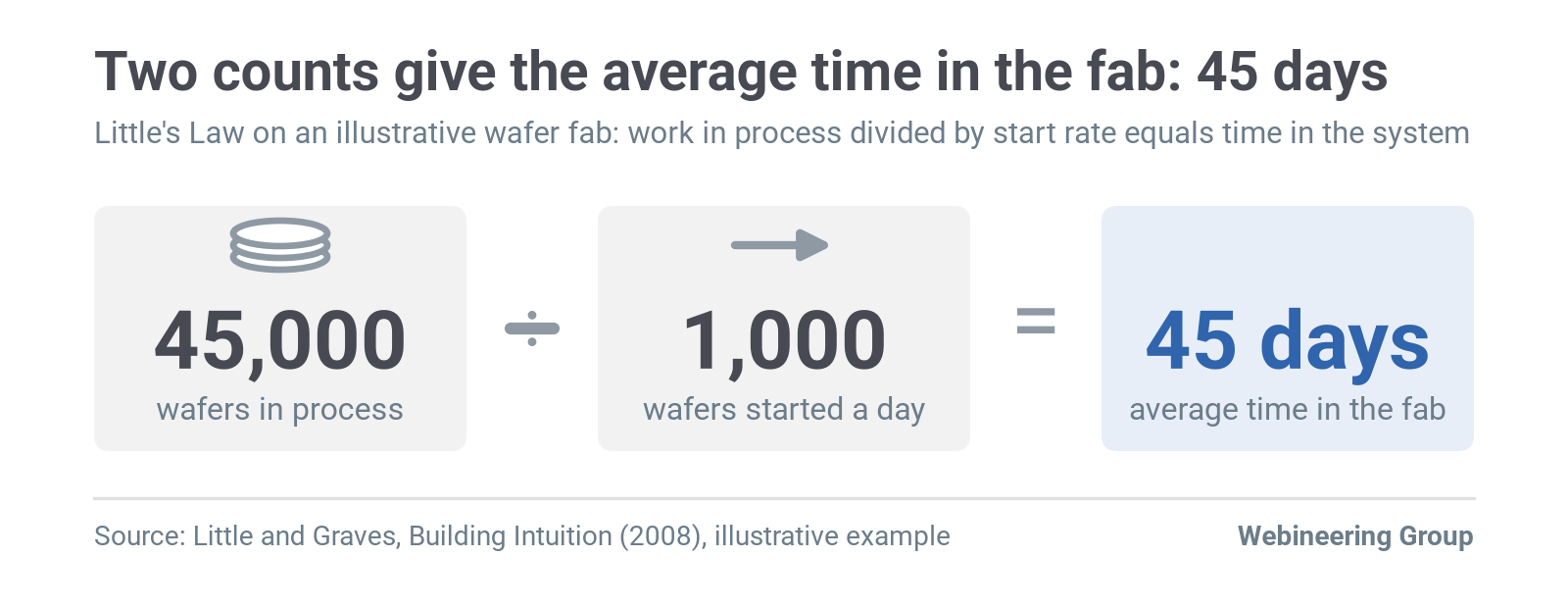
John Little and Stephen Graves of MIT give a clean example in their chapter on Little's Law in Building Intuition (Springer, 2008). In their illustrative case, a semiconductor fab holds an average of 45,000 wafers in process and starts 1,000 wafers a day. That start rate has held steady for nine months, so average time in the fab is 45 days.
The example needs only two counts a plant already keeps: wafers in process and starts per day. The same arithmetic works on your floor, where the two counts are open jobs and weekly shipments. Little and Graves call this kind of use a back-of-the-envelope calculation: two of the terms are easy to estimate, and the law supplies the third.
Benchmarks for process cycle efficiency disagree
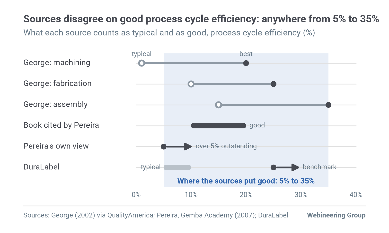
Common advice says to compare your process cycle efficiency with a published benchmark for the best plants. The usual source is Michael George's Lean Six Sigma (McGraw-Hill, 2002), as reproduced by QualityAmerica. For typical plants against the best, it lists machining at 1% against 20%, fabrication at 10% against 25%, and assembly at 15% against 35%.
Other sources set the bar elsewhere. Ron Pereira of Gemba Academy wrote in March 2007 that one popular book calls 10% to 20% good, while others set the top mark at 5% and above.
His own view, from experience, is that a figure over 5% is "outstanding" for discrete manufacturing. DuraLabel, a label vendor, presents 5% to 10% as typical and more than 25% as the lean benchmark.
Part of the gap comes from definitions. Rui Sousa, José Dinis-Carvalho and Peter Hines, in Production Engineering Archives in 2026, name confusion between value-added, processing and cycle time as a recurring mapping problem. They add confusion between process lead time and inventory lead time.
Two plants with different boundaries and units can't share a benchmark, so measure your own number the same way every time and watch its trend. A ratio measured on one family tells you more about that family than any published table does, and a monthly trend on the same boundary shows whether queues are shrinking.
Fix your boundary before you count: release-to-ship is a good default for job shops because both ends leave a date in the system, and both are easy to audit. Write the boundary on the sheet so next quarter's count matches this one. If engineering release comes before material arrives, start the clock at material release and note that choice on the sheet.
Manufacturing lead time calculation in five days
Little's Law says average work in process equals the exit rate times average time in the system. Wallace Hopp and Mark Spearman treat it as a fundamental relationship in Factory Physics, first published in 1996. It holds for long-run averages in a stable system, so the steps below use a quarter of output.
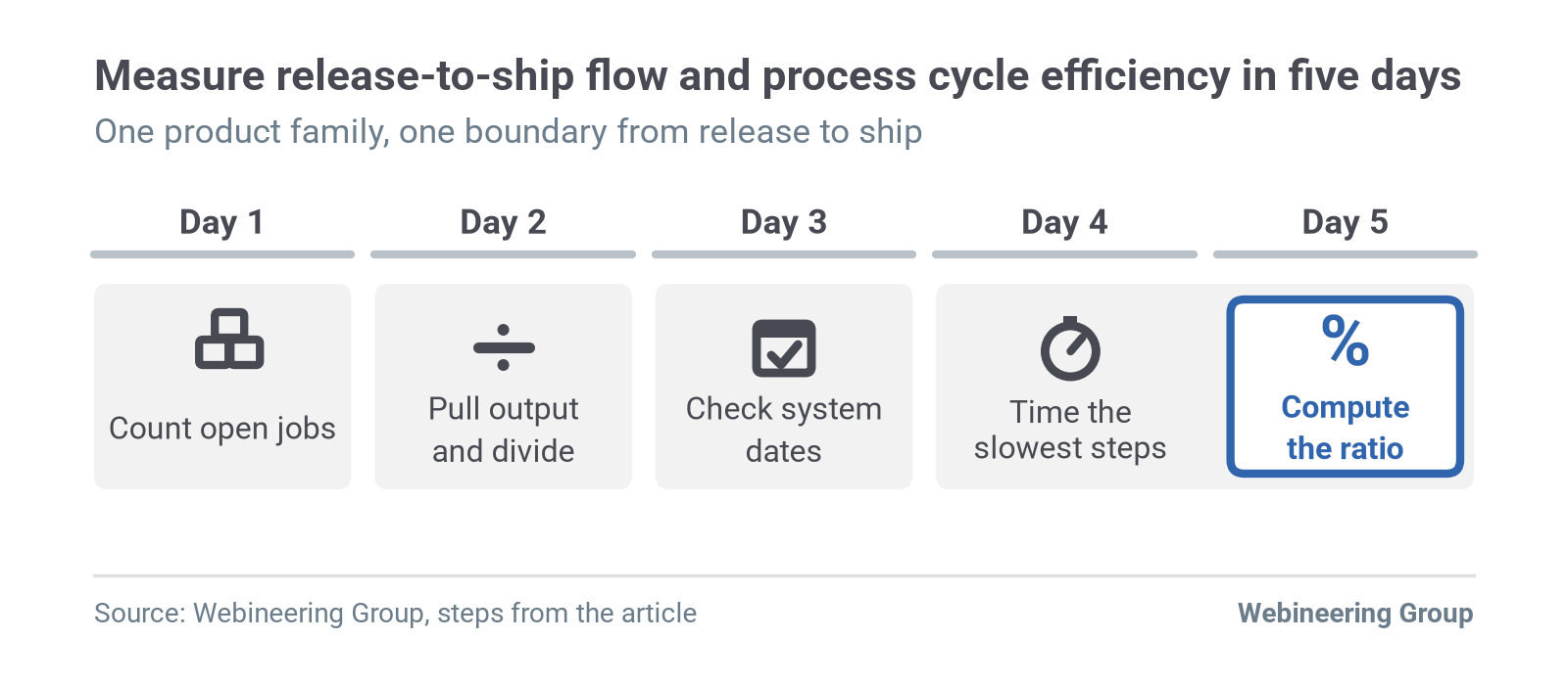
- Day one: count the work in process. Pick one product family and count every open job between release and ship on one day, including jobs waiting in engineering, scheduling or on hold. The Rolls-Royce supplier value stream mapping guide (2020) tells suppliers to "count the actual inventory at each stage of the process."
- Day two: pull weekly output. Average the jobs shipped per week for that family over the last 8 to 13 weeks. Use shipped jobs, because a job counts as output only when it leaves the boundary.
- Day two: divide. Lead time in weeks equals work in process divided by weekly output.
- Day three: cross-check with system dates. Export release and ship dates for jobs closed last month from your enterprise resource planning (ERP) system. Report the median and the 85th percentile in working days, and keep only the shop floor data fields you trust.
- Days four and five: correct the touch time. Sum touch time from routings, then time two or three jobs at their slowest steps. Replace routing standards with observed minutes where they differ.
- Day five: compute process cycle efficiency. Divide value-added time by lead time in matching units.
A worked example lands at 3.5%
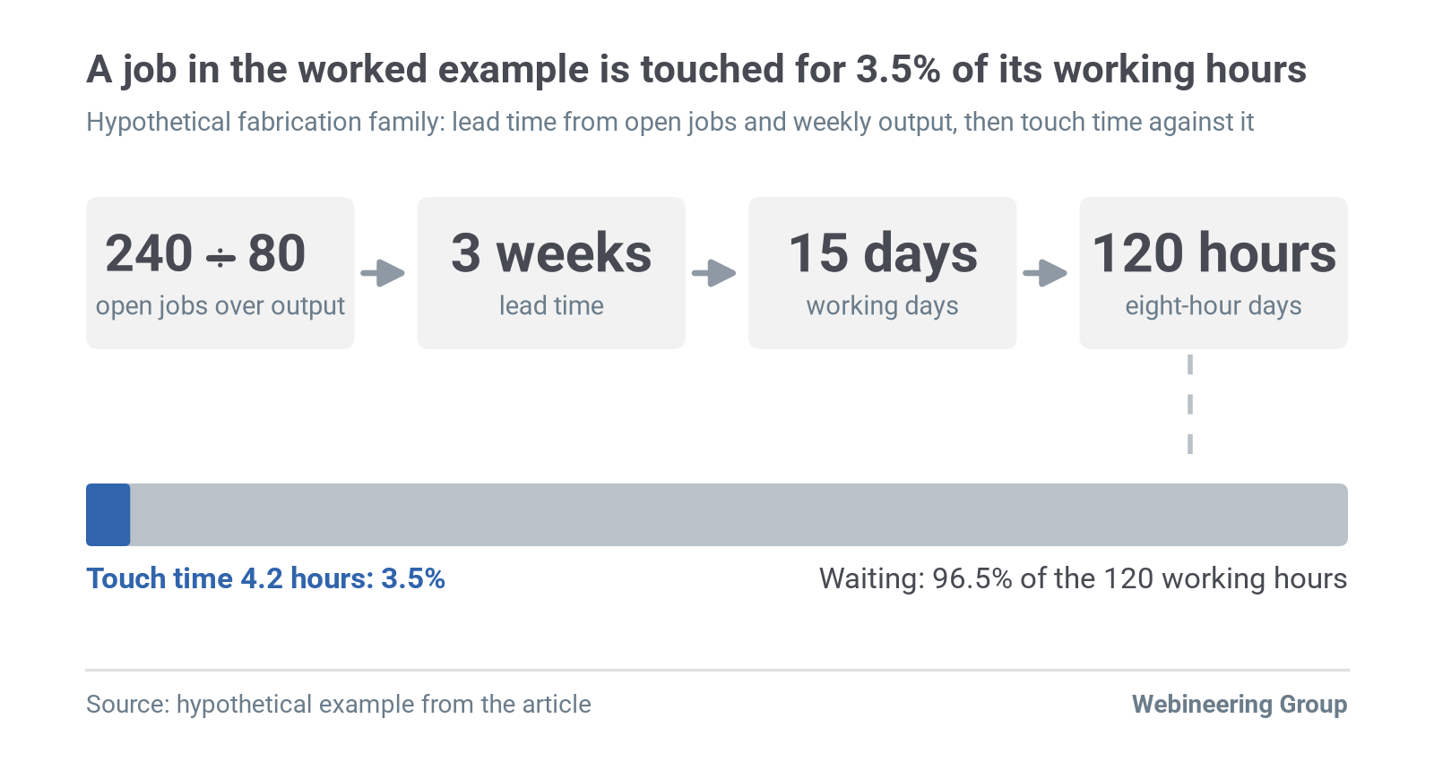
Picture a hypothetical fabrication family with 240 open jobs between release and ship and average output of 80 jobs a week over 13 weeks. Lead time is 240 ÷ 80 = 3 weeks, or 15 working days. System dates give a median of 14 working days and an 85th percentile of 22, so the estimate holds and the tail is long.
Routings say 3.5 hours of touch time, and timing two jobs moves it to 4.2 hours.
On eight-hour working days, lead time is 120 working hours, so process cycle efficiency is 4.2 ÷ 120 = 3.5%. For 96.5% of its working hours in the flow, a job waits. A ratio that low is common: George's table puts typical machining at 1%.
Read the gap between the median and the 85th percentile as a scheduling signal. When the tail runs eight working days past the median, some jobs are waiting on priorities, material or approvals that the routing never shows. Pull the five slowest jobs from last month and trace where each one sat. Those five jobs show where the queue time sits.
Start with jobs that cross a shift change. A shift handover report that names every waiting job shows where they sit.
Five errors distort the value added ratio
Each error below moves the number in one direction, so check all five before you report a figure to anyone.
| Error | What it does to the number | Fix |
|---|---|---|
| Mixing calendar and working days | Inflates lead time by 40% on a five-day week (7 ÷ 5) | Put both terms in working days or working hours |
| Routing standards used as touch time | Misstates value-added time when practice has drifted | Time two or three jobs and correct the sum |
| Counting only floor work in process | Understates lead time when jobs wait in engineering or scheduling | Count from release, wherever the job sits |
| Little's Law applied when output runs well below demand | Output reflects a constraint, and the backlog grows outside the count | Use stable weeks only, or count the backlog too |
| A step's whole cycle time counted as value-added | Inflates process cycle efficiency | Count only minutes that change the product |
Four conditions break the estimate
- Unstable output. Ramp-up, a shutdown week or a growing backlog breaks the long-run average Little's Law needs, so wait for stable weeks or count the backlog.
- Continuous process plants. Work in process sits in tanks and pipes, so measure volume and flow rate in matching units.
- Engineer-to-order work. Release-to-ship includes design time, so split design from build and measure each.
- A ratio that moves for the wrong reasons. A slower step adds touch minutes and lifts process cycle efficiency while customers wait just as long. The mirror case holds too: cut touch time faster than lead time and the ratio falls even as the work improves. Report the ratio next to lead time every time.
Start these five on Monday
- Count every open job between release and ship for one product family.
- Pull weekly shipments for that family for the last quarter.
- Divide work in process by weekly output.
- Export release and ship dates for jobs closed last month.
- Time two jobs at their slowest step.
Get your release-to-ship number measured
Webineering's fixed-fee site assessment reviews floor processes, records and reports for one value stream. Its one written report includes release-to-ship lead time and value-added share for that value stream, and we use the same counts this article walks through.
Site assessment
Want to see where your own line stands?
An evidence-backed report on where real value lies, from the people who stay through implementation.
Authors
Anthony Occidentale
Principal
Founder